1	2	3	4	5	6	7	8	9	10	11	12	13	14
1		23			54		55				26			
2	23		56		18									
3		56		50	44	61								
4			50			28				27				
5	54	18	44			51	34	56	48					
6			61	28	51				27	42				
7	55				34			36				38		
8					56		36		29			33		
9					48	27		29		61		29	42	36
10				27		42			61					25
11	26											24		
12							38	33	29		24		30	
13									42			30		47
14									36	25			47	

import numpy as np
import pandas as pd
from scipy.sparse import coo_matrix
import networkx as nx
import matplotlib.pyplot as plt

"""
numpy: 1.24.3
pandas: 1.5.3
networkx: 3.1
matplotlib: 3.7.5
"""

# 避免图片无法显示中文
plt.rcParams['font.sans-serif'] = ['SimHei']
# 显示所有列
pd.set_option('display.max_columns', None)
pd.set_option('display.width', 1000)

# 读取数据
dataframe = pd.read_excel(io='data.xlsx', sheet_name='Sheet1', index_col=0)
dataframe = dataframe.fillna(0)
print('矩阵的空值以0填充：\n', dataframe)
coo = coo_matrix(np.array(dataframe))
# 矩阵行列的索引默认从0开始改成从1开始
coo.row += 1
coo.col += 1
data = [int(i) for i in coo.data]
coo_tuple = list(zip(coo.row, coo.col, data))
coo_list = []
for i in coo_tuple:
    coo_list.append(list(i))

# 出发点
start_node = 1
# 目的地
target_node = 14
# 设置各顶点坐标（只是方便绘图，并不是实际位置）
pos = {1: (1, 8), 2: (4, 10), 3: (11, 11), 4: (14, 8), 5: (5, 7), 6: (10, 6), 7: (3, 5), 8: (6, 4), 9: (8, 4),
       10: (14, 5), 11: (2, 3), 12: (5, 1), 13: (8, 1), 14: (13, 3)}

# 创建空的无向图
G = nx.Graph()
# 给无向图的边赋予权值
G.add_weighted_edges_from(coo_list)

# 单源最短路径dijkstra迪杰斯特拉算法求最短路径和最短路程
min_path_dijkstra = nx.dijkstra_path(G, source=start_node, target=target_node)
min_path_length_dijkstra = nx.dijkstra_path_length(G, source=start_node, target=target_node)
print('\ndijkstra算法：顶点%d到顶点%d的最短路径:%s，最短路程:%d' % (
    start_node, target_node, min_path_dijkstra, min_path_length_dijkstra))

# 单源最短路径bellman-ford贝尔曼-福特算法求最短路径和最短路程
min_path_bellman_ford = nx.bellman_ford_path(G, source=start_node, target=target_node)
min_path_length_bellman_ford = nx.bellman_ford_path_length(G, source=start_node, target=target_node)
print('\nbellman-ford算法：顶点%d到顶点%d的最短路径:%s，最短路程:%d' % (
    start_node, target_node, min_path_bellman_ford, min_path_length_bellman_ford))

# 单源最短路径A*算法求最短路径和最短路程
min_path_astar = nx.astar_path(G, source=start_node, target=target_node)
min_path_length_astar = nx.astar_path_length(G, source=start_node, target=target_node)
print('\nA*算法：顶点%d到顶点%d的最短路径:%s，最短路程:%d' % (
    start_node, target_node, min_path_astar, min_path_length_astar))

# 多源最短路径floyd弗洛伊德算法求最短路径和最短路程
min_path_floyd, _ = nx.floyd_warshall_predecessor_and_distance(G)
min_path_length_floyd = nx.floyd_warshall_numpy(G)
min_path_length_floyd = pd.DataFrame(data=min_path_length_floyd, index=dataframe.index, columns=dataframe.columns)
print('\nfloyd算法：顶点%d到顶点%d的最短路径:%s，最短路程:%d' % (
    start_node, target_node, nx.reconstruct_path(start_node, target_node, min_path_floyd),
    min_path_length_floyd[start_node][target_node]))

# 多源最短路径johnson约翰逊算法求最短路径和最短路程
min_path_johnson = nx.johnson(G)
print('\njohnson算法：顶点%d到顶点%d的最短路径:%s' % (
    start_node, target_node, min_path_johnson[start_node][target_node]))  # networkx库没有专门针对johnson算法求最短路程的模块

plt.figure()
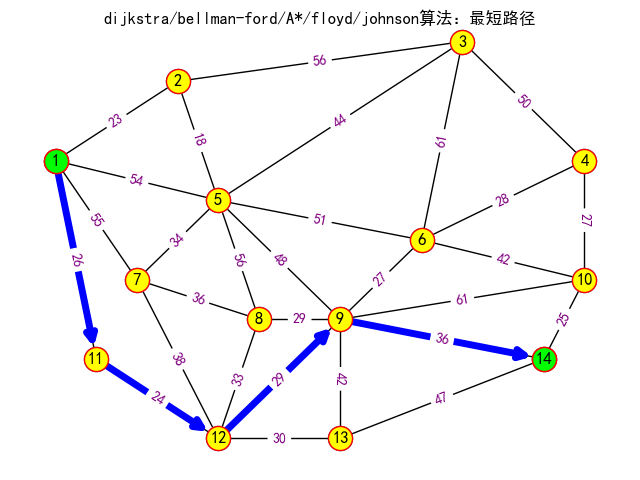
plt.suptitle('dijkstra/bellman-ford/A*/floyd/johnson算法：最短路径')
# 绘制无向加权图
nx.draw(G, pos, with_labels=True)
# 设置顶点颜色
nx.draw_networkx_nodes(G, pos, nodelist=G.nodes, node_color='yellow', edgecolors='red')
# 设置最短路径的边颜色、宽度、箭头效果
nx.draw_networkx_edges(G, pos, edgelist=[[min_path_dijkstra[i], min_path_dijkstra[i + 1]] for i in
                                         range(len(min_path_dijkstra) - 1)], edge_color='blue', width=5, arrows=True,
                       arrowstyle='->', arrowsize=15)
# 显示无向加权图的边的权值
labels = nx.get_edge_attributes(G, 'weight')
# 显示边的权值
nx.draw_networkx_edge_labels(G, pos, edge_labels=labels, font_color='purple', font_size=10)
nx.draw_networkx_nodes(G, pos, nodelist=[start_node, target_node], node_color='#00ff00', edgecolors='red')
plt.show()

矩阵的空值以0填充：
       1     2     3     4     5     6     7     8     9     10    11    12    13    14
1    0.0  23.0   0.0   0.0  54.0   0.0  55.0   0.0   0.0   0.0  26.0   0.0   0.0   0.0
2   23.0   0.0  56.0   0.0  18.0   0.0   0.0   0.0   0.0   0.0   0.0   0.0   0.0   0.0
3    0.0  56.0   0.0  50.0  44.0  61.0   0.0   0.0   0.0   0.0   0.0   0.0   0.0   0.0
4    0.0   0.0  50.0   0.0   0.0  28.0   0.0   0.0   0.0  27.0   0.0   0.0   0.0   0.0
5   54.0  18.0  44.0   0.0   0.0  51.0  34.0  56.0  48.0   0.0   0.0   0.0   0.0   0.0
6    0.0   0.0  61.0  28.0  51.0   0.0   0.0   0.0  27.0  42.0   0.0   0.0   0.0   0.0
7   55.0   0.0   0.0   0.0  34.0   0.0   0.0  36.0   0.0   0.0   0.0  38.0   0.0   0.0
8    0.0   0.0   0.0   0.0  56.0   0.0  36.0   0.0  29.0   0.0   0.0  33.0   0.0   0.0
9    0.0   0.0   0.0   0.0  48.0  27.0   0.0  29.0   0.0  61.0   0.0  29.0  42.0  36.0
10   0.0   0.0   0.0  27.0   0.0  42.0   0.0   0.0  61.0   0.0   0.0   0.0   0.0  25.0
11  26.0   0.0   0.0   0.0   0.0   0.0   0.0   0.0   0.0   0.0   0.0  24.0   0.0   0.0
12   0.0   0.0   0.0   0.0   0.0   0.0  38.0  33.0  29.0   0.0  24.0   0.0  30.0   0.0
13   0.0   0.0   0.0   0.0   0.0   0.0   0.0   0.0  42.0   0.0   0.0  30.0   0.0  47.0
14   0.0   0.0   0.0   0.0   0.0   0.0   0.0   0.0  36.0  25.0   0.0   0.0  47.0   0.0

dijkstra算法：顶点1到顶点14的最短路径:[1, 11, 12, 9, 14]，最短路程:115

bellman-ford算法：顶点1到顶点14的最短路径:[1, 11, 12, 9, 14]，最短路程:115

A*算法：顶点1到顶点14的最短路径:[1, 11, 12, 9, 14]，最短路程:115

floyd算法：顶点1到顶点14的最短路径:[1, 11, 12, 9, 14]，最短路程:115

johnson算法：顶点1到顶点14的最短路径:[1, 11, 12, 9, 14]