Scikit Opt库的学习历程:免疫优化算法
4 min read
Page Views
1.原始数据
现有100个坐标点,范围在0~100之间,数据如下所示:
| X轴 | Y轴 |
|---|---|
| 34.42003055 | 15.09116107 |
| 65.62884169 | 41.19011147 |
| 19.78223979 | 5.42221394 |
| 20.53506676 | 61.13539415 |
| 6.938172809 | 57.29011679 |
| 15.65276333 | 92.75947909 |
| 82.57833045 | 91.01977119 |
| 34.61285576 | 69.90342925 |
| 73.45539957 | 49.74808012 |
| 11.1618541 | 10.61982769 |
| 17.90187451 | 97.84619374 |
| 67.93421171 | 27.2838889 |
| 53.62705292 | 26.14745172 |
| 98.54491062 | 39.6049835 |
| 77.93630214 | 83.46127415 |
| 34.57561112 | 73.46294865 |
| 81.99432822 | 36.84855934 |
| 75.74345312 | 72.80338896 |
| 7.122473935 | 69.18779138 |
| 67.01118709 | 7.210402341 |
| 51.95833187 | 99.32382751 |
| 38.79375773 | 23.93629424 |
| 99.81463149 | 61.6275386 |
| 99.81818868 | 20.5606421 |
| 70.70990641 | 81.30779579 |
| 95.23801276 | 76.6939803 |
| 66.32296759 | 66.30345872 |
| 43.69979358 | 73.54613243 |
| 2.60386653 | 29.70693259 |
| 41.14812876 | 16.09362293 |
| 57.76582018 | 47.33432892 |
| 71.5123502 | 46.49765388 |
| 91.25640584 | 39.69177854 |
| 60.17074572 | 12.45320955 |
| 55.62170552 | 55.90896433 |
| 98.78427702 | 99.92598117 |
| 43.07126016 | 99.82299762 |
| 71.07448958 | 93.97100808 |
| 32.01786582 | 46.43916948 |
| 11.33400935 | 76.68578456 |
| 39.89722972 | 87.88671429 |
| 45.33051316 | 62.81179907 |
| 44.64643445 | 61.87150901 |
| 54.57135064 | 1.526391294 |
| 10.0995678 | 62.48269012 |
| 57.14681548 | 39.89805412 |
| 96.64454834 | 84.62722077 |
| 56.07897662 | 95.11254919 |
| 20.90569065 | 53.47336942 |
| 10.77890818 | 0.450097076 |
| 58.27668885 | 17.81198283 |
| 13.7944935 | 44.29804004 |
| 56.34877372 | 99.21893791 |
| 13.56813317 | 67.72809972 |
| 27.78243926 | 92.64794811 |
| 24.0975343 | 5.80169803 |
| 8.838345877 | 80.98711459 |
| 10.11576809 | 96.17782143 |
| 74.63305732 | 49.87126999 |
| 89.3467241 | 94.22295884 |
| 41.14605604 | 68.92348595 |
| 26.35508285 | 27.13734184 |
| 58.9166891 | 47.53662527 |
| 49.4740803 | 18.23096755 |
| 72.62774707 | 97.47410575 |
| 91.48393926 | 56.46157428 |
| 19.09762019 | 74.87408524 |
| 95.84089078 | 11.23002409 |
| 53.72913752 | 76.94628201 |
| 4.953191672 | 36.85663429 |
| 22.16789385 | 91.03424379 |
| 10.43448424 | 44.41017144 |
| 82.18757767 | 44.12566975 |
| 12.20174646 | 14.61619704 |
| 61.44310703 | 40.11938774 |
| 23.97419787 | 21.55870951 |
| 4.6524454 | 52.56070117 |
| 85.69261457 | 24.9662534 |
| 35.33504583 | 69.49180995 |
| 95.64301042 | 51.32300182 |
| 0.698648231 | 61.01585057 |
| 36.32208842 | 44.48727401 |
| 39.33287013 | 19.95496495 |
| 28.36904573 | 73.57055232 |
| 74.46852466 | 95.76737957 |
| 69.32584873 | 42.80289419 |
| 39.19680184 | 40.17020467 |
| 75.12636314 | 17.99013581 |
| 97.70317034 | 83.85365282 |
| 1.763900929 | 75.11858627 |
| 68.22594191 | 72.26483955 |
| 29.34328245 | 23.97405157 |
| 31.80158588 | 6.647953798 |
| 65.98598209 | 64.39250268 |
| 12.60662276 | 75.51809864 |
| 11.17410019 | 50.82785738 |
| 47.34378637 | 81.26562912 |
| 37.39671811 | 34.26505211 |
| 24.55262347 | 28.00817421 |
| 3.98159549 | 22.32023408 |
2.python程序
import numpy as np
import pandas as pd
from scipy import spatial
from sko.IA import IA_TSP
import matplotlib.pyplot as plt

"""
numpy: 1.24.3
pandas: 1.5.3
scipy: 1.10.1
scikit-opt 0.6.6
sko 0.5.7
matplotlib: 3.7.5
"""

plt.rcParams['font.sans-serif'] = ['SimHei']
plt.rcParams['axes.unicode_minus'] = False

# 参数设置
num_points = 100
size_pop = 100
max_iter = 5000

# 读取坐标信息
points = pd.read_excel('数据.xlsx')
points_coordinate = np.array(points.values.tolist())
distance_matrix = spatial.distance.cdist(points_coordinate, points_coordinate, metric='euclidean')

def cal_total_distance(routine):
    num_points, = routine.shape
    return sum([distance_matrix[routine[i % num_points], routine[(i + 1) % num_points]] for i in range(num_points)])

# 初始化免疫优化算法算法
ia_tsp = IA_TSP(func=cal_total_distance, n_dim=num_points, size_pop=size_pop, max_iter=max_iter, prob_mut=0.2,
                T=0.7, alpha=0.95)

# 创建图形
fig, (ax1, ax2) = plt.subplots(1, 2, figsize=(12, 6))
fig.suptitle('基于免疫优化算法求解旅行商问题')

# 路线图设置
ax1.set_title('旅行商路线图')
ax1.set_xlim(0, 100)
ax1.set_ylim(0, 100)
ax1.set_xlabel('X轴')
ax1.set_ylabel('Y轴')
ax1.set_aspect('equal')

# 收敛曲线图设置
ax2.set_title('收敛曲线图')
ax2.set_xlabel('迭代次数')
ax2.set_ylabel('总里程数')
ax2.grid(True)
ax2.set_xlim(0, max_iter)
ax2.set_aspect('auto')

# 初始化图形元素
line, = ax1.plot([], [], 'o-r', markersize=4, linewidth=1)
scatter = ax1.scatter(points_coordinate[:, 0], points_coordinate[:, 1], c='r', s=20)
convergence_line, = ax2.plot([], [], 'b-', linewidth=2)
best_distance_text = ax2.text(0.75, 0.75, '', transform=ax2.transAxes)

# 计算y轴范围
initial_distance = cal_total_distance(np.arange(num_points))
ax2.set_ylim(0, initial_distance * 1.1)

# 生成最后迭代结果
best_points, best_distance = ia_tsp.run()
best_points_ = np.concatenate([best_points, [best_points[0]]])
best_points_coordinate = points_coordinate[best_points_, :]
ax1.plot(best_points_coordinate[:, 0], best_points_coordinate[:, 1], 'o-r')
ax2.plot(ia_tsp.generation_best_Y)
best_distance_text.set_text(f'迭代次数:{max_iter}\n\n总里程数:{best_distance[-1]:.2f}')
plt.tight_layout()
plt.show()
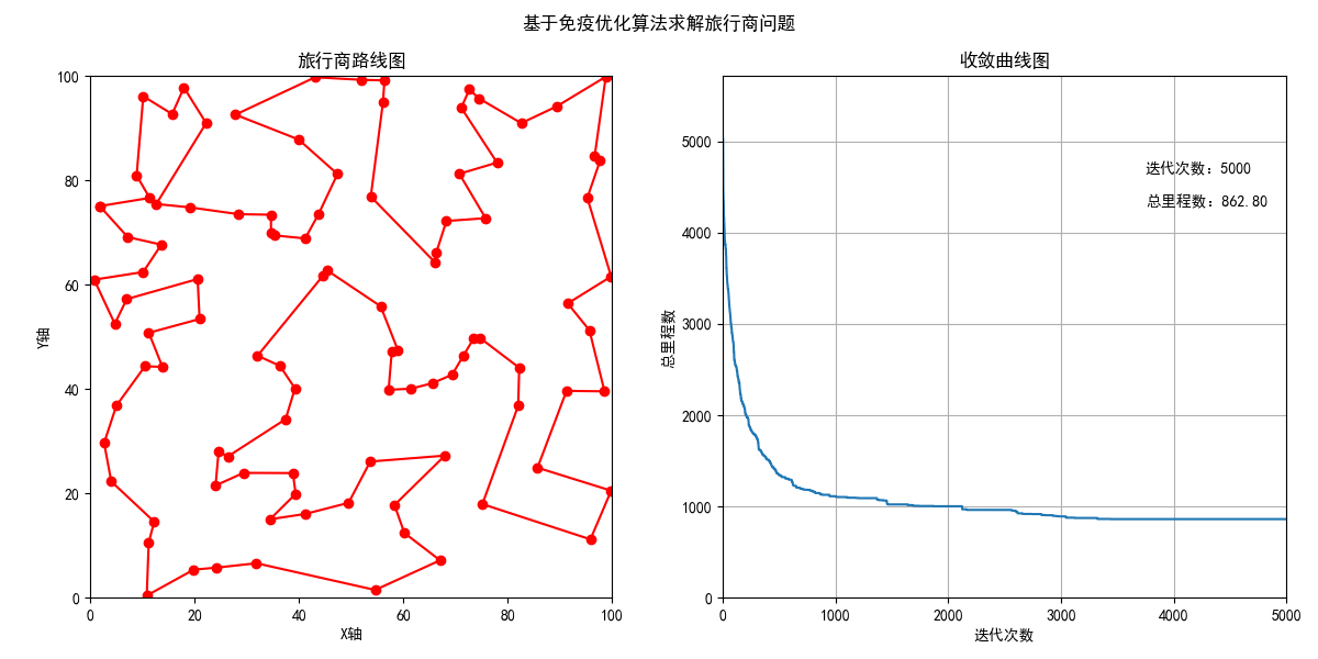
3.效果展示
Last updated on 2025-05-29